Part III: Diversity and similarity of repertoires
In this part the repertoire similarity in terms of the number of unique overlapping clonotypes and their frequency is calculated, termed overlap-D and overlap-F respectively. Datasets used in this part are the same as ones in Part II.
Computing pairwise similarities
As computing pairwise overlaps is either memory-demanding (in case we load all samples into memory) or slow (loading only one pair at a time), we will first down-sample datasets to 50,000 cells each.
$VDJTOOLS Downsample -x 50000 -m ../part2/metadata.txt .
Next we will compute pairwise similarities
$VDJTOOLS CalcPairwiseDistances -i aa\!nt -m metadata.txt .
Important
Here we apply the aa!nt clonotype matching rule, which means that clonotypes match when their CDR3 amino acid sequences match, but nucleotide sequences are different. This rule is effective agains cross-sample contamination, which is an issue in analyzed datasets as they were prepared in three separate batches (A2, A3 and A4)
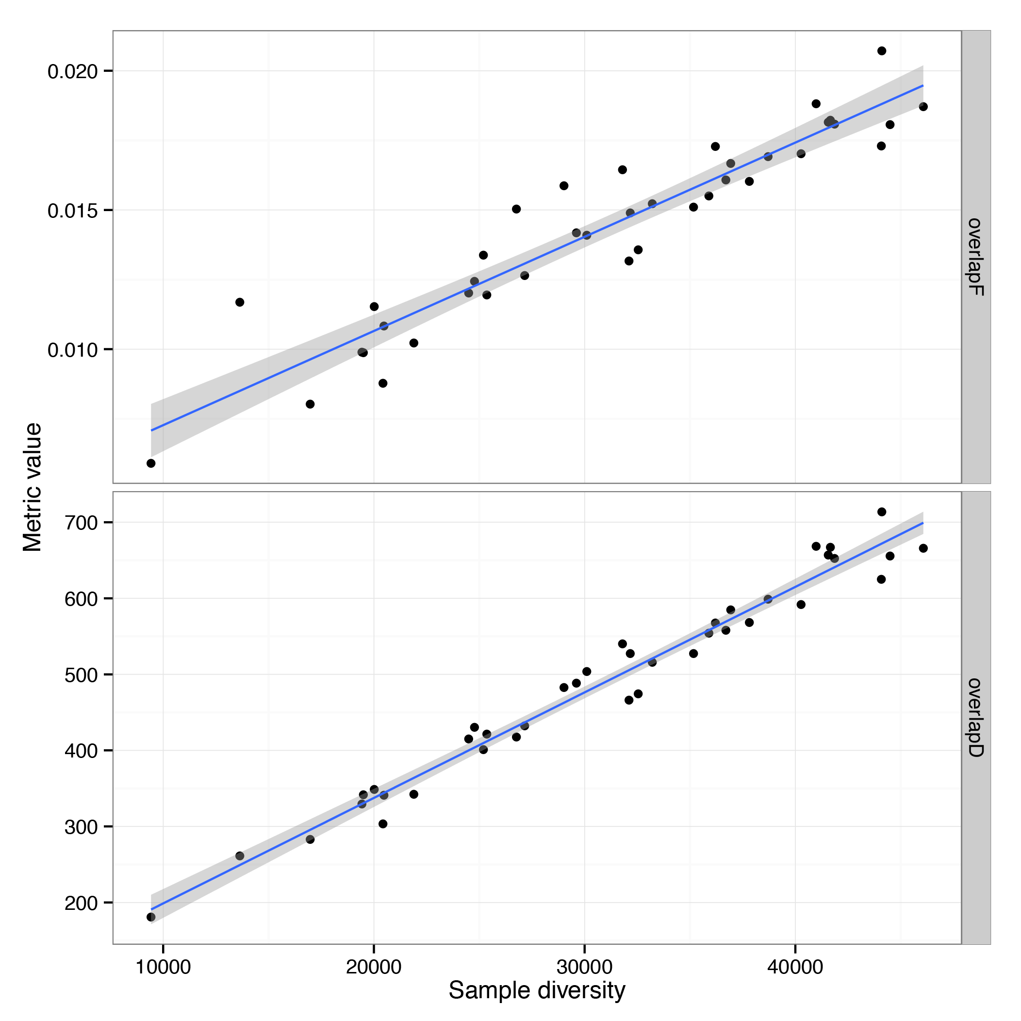
Correlation between overlap and diversity
Run the following script to compute and plot the relation between sample diversity and its mean overlap with other samples
require(ggplot2); require(plyr); require(reshape)

# load table
df <- read.table("intersect.batch.aa!nt.txt", header=T, sep="\t", comment="")

df$F2 <- as.numeric(as.character(df$F2))

# need to do this, as only the upper triangular of intersection matrix is stored
df.1 <- rbind(data.frame(sample=df$X.1_sample_id, div=df$div1, overlapF=df$F2, overlapD=df$div12),
              data.frame(sample=df$X2_sample_id, div=df$div2, overlapF=df$F2, overlapD=df$div12))

# compute mean values for overlap-F and -D
df.2 <- ddply(df.1, .(sample), summarise,
              div=mean(div),
              overlapF=mean(overlapF),
              overlapD=mean(overlapD))

# plot
df.3 <- melt(df.2, id=c("sample","div"))

pdf("overlap.pdf")
ggplot(df.3, aes(x=div,y=value)) + geom_point() + geom_smooth(method=lm) +
  xlab("Sample diversity") + ylab("Metric value") +
  facet_grid(variable~.,scales="free_y") + theme_bw()
dev.off()
Note
More diverse samples are actually highly similar, both in terms of unique clonotypes in the overlap and total overlap frequency.
Next, lets cluster samples based on their similarity,
$VDJTOOLS ClusterSamples -e F2 -i aa\!nt -f age -n -p .
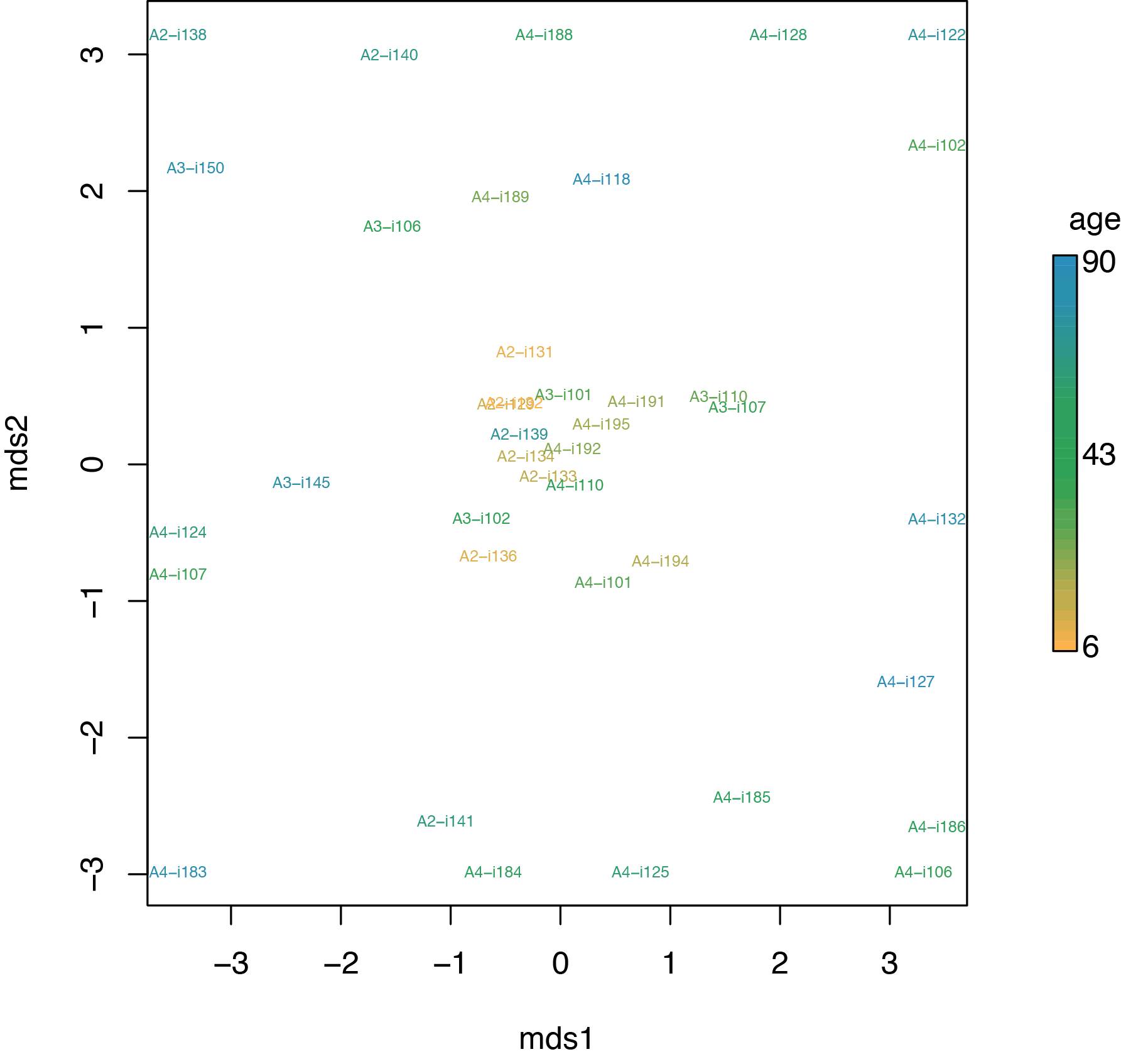
This will generate hc*.pdf with hierarchical clustering and mds*.pdf
with multi-dimensional scaling plots.
Note
The MDS plot show that younger and more diverse repertoires are more similar than elder repertoires. From immunological point of view given additional data on umbilical cord blood repertoires and elder individuals (not shown here), this is interpreted in the following way:
We are born with highly similar, convergent and evolutionary optimized repertoires, but random clonal expansion (partially due to T-cell cross-reactivity) decrease the overlap between our repertoires.